Pandas and Friends
What does it do?
Pandas is a Python data analysis tool built on top of NumPy that provides a suite of data structures and data manipulation functions to work on those data structures. It is particularly well suited for working with time series data.
Getting Started - Installation
Installing with pip or apt-get::
pip install pandas
# or
sudo apt-get install python-pandas
- Mac - Homebrew or MacPorts to get the dependencies, then pip
- Windows - Python(x,y)?
- Commercial Pythons: Anaconda, Canopy
Getting Started - Dependencies
Dependencies, required, recommended and optional
# Required
numpy, python-dateutil, pytx
# Recommended
numexpr, bottleneck
# Optional
cython, scipy, pytables, matplotlib, statsmodels, openpyxl
Pandas’ Friends!
Pandas works along side and is built on top of several other Python projects.
-
IPython
-
Numpy
-
Matplotlib
Pandas gets along with EVERYONE!
Background - IPython
IPython is a fancy python console. Try running ipython or ipython --pylab on your command line. Some IPython tips
# Special commands, 'magic functions', begin with %
%quickref, %who, %run, %reset
# Shell Commands
ls, cd, pwd, mkdir
# Need Help?
help(), help(obj), obj?, function?
# Tab completion of variables, attributes and methods
Background - IPython Notebook
There is a web interface to IPython, known as the IPython notebook, start it like this
ipython notebook
# or to get all of the pylab components
ipython notebook --pylab
IPython - Follow Along
Follow along by connecting to TMPNB.ORG!
Background - NumPy
- NumPy is the foundation for Pandas
- Numerical data structures (mostly Arrays)
- Operations on those.
- Less structure than Pandas provides.
Background - NumPy - Arrays
import numpy as np
# np.zeros, np.ones
data0 = np.zeros((2, 4))

data0

array([[ 0.,  0.,  0.,  0.],
       [ 0.,  0.,  0.,  0.]])

# Make an array with 20 entries 0..19
data1 = np.arange(20)
# print the first 8
data1[0:8]

array([0, 1, 2, 3, 4, 5, 6, 7])
Background - NumPy - Arrays
# make it a 4,5 array
data = np.arange(20).reshape(4, 5)
data

array([[ 0,  1,  2,  3,  4],
       [ 5,  6,  7,  8,  9],
       [10, 11, 12, 13, 14],
       [15, 16, 17, 18, 19]])
Background - NumPy - Arrays
Arrays have NumPy specific types, dtypes, and can be operated on.
print("dtype: ", data.dtype)
result = data * 20.5
print(result)

('dtype: ', dtype('int64'))
[[   0.    20.5   41.    61.5   82. ]
 [ 102.5  123.   143.5  164.   184.5]
 [ 205.   225.5  246.   266.5  287. ]
 [ 307.5  328.   348.5  369.   389.5]]
Now, on to Pandas
Pandas
- Tabular, Timeseries, Matrix Data - labeled or not
- Sensible handling of missing data and data alignment
- Data selection, slicing and reshaping features
- Robust data import utilities.
- Advanced time series capabilities
Data Structures
- Series - 1D labeled array
- DataFrame - 2D labeled array
- Panel - 3D labeled array (More D)
Assumed Imports
In my code samples, assume I import the following
import pandas as pd
import numpy as np
Series
- one-dimensional labeled array
- holds any data type
- axis labels known as index
- implicit integert indexes
dict-like
Create a Simple Series
s1 = pd.Series([1, 2, 3, 4, 5])
s1

0    1
1    2
2    3
3    4
4    5
dtype: int64
Series Operations
# integer multiplication
print(s1 * 5)

0     5
1    10
2    15
3    20
4    25
dtype: int64
Series Operations - Cont.
# float multiplication
print(s1 * 5.0)

0     5
1    10
2    15
3    20
4    25
dtype: float64
Series Index
s2 = pd.Series([1, 2, 3, 4, 5],
               index=['a', 'b', 'c', 'd', 'e'])
s2

a    1
b    2
c    3
d    4
e    5
dtype: int64
Date Convenience Functions
A quick aside …
dates = pd.date_range('20130626', periods=5)
print(dates)
print()
print(dates[0])

<class 'pandas.tseries.index.DatetimeIndex'>
[2013-06-26, ..., 2013-06-30]
Length: 5, Freq: D, Timezone: None
()
2013-06-26 00:00:00
Datestamps as Index
s3 = pd.Series([1, 2, 3, 4, 5], index=dates)
print(s3)

2013-06-26    1
2013-06-27    2
2013-06-28    3
2013-06-29    4
2013-06-30    5
Freq: D, dtype: int64
Selecting By Index
Note that the integer index is retained along with the new date index.
print(s3[0])
print(type(s3[0]))
print()
print(s3[1:3])
print(type(s3[1:3]))

1
<type 'numpy.int64'>
()
2013-06-27    2
2013-06-28    3
Freq: D, dtype: int64
<class 'pandas.core.series.Series'>
Selecting by value
s3[s3 < 3]

2013-06-26    1
2013-06-27    2
Freq: D, dtype: int64
Selecting by Label (Date)
s3['20130626':'20130628']

2013-06-26    1
2013-06-27    2
2013-06-28    3
Freq: D, dtype: int64
Series Wrapup
Things not covered but you should look into:
- Other instantiation options:
dict - Operator Handling of missing data
NaN - Reforming Data and Indexes
- Boolean Indexing
-
Other Series Attributes:
index-index.namename- Series name
DataFrame
- 2-dimensional labeled data structure
- Like a SQL Table, Spreadsheet or
dictofSeriesobjects. - Columns of potentially different types
- Operations, slicing and other behavior just like
Series
DataFrame - Simple
data1 = pd.DataFrame(np.random.rand(4, 4))
data1
| 0 | 1 | 2 | 3 | |
|---|---|---|---|---|
| 0 | 0.002581 | 0.851980 | 0.097265 | 0.648841 |
| 1 | 0.732965 | 0.820690 | 0.895176 | 0.582483 |
| 2 | 0.176504 | 0.068942 | 0.466759 | 0.918777 |
| 3 | 0.938426 | 0.097954 | 0.696534 | 0.684424 |
DataFrame - Index/Column Names
dates = pd.date_range('20130626', periods=4)
data2 = pd.DataFrame(
    np.random.rand(4, 4),
    index=dates, columns=list('ABCD'))
data2
| A | B | C | D | |
|---|---|---|---|---|
| 2013-06-26 | 0.831222 | 0.209279 | 0.340186 | 0.928447 |
| 2013-06-27 | 0.252513 | 0.452392 | 0.862822 | 0.738837 |
| 2013-06-28 | 0.309083 | 0.822918 | 0.924720 | 0.964607 |
| 2013-06-29 | 0.827998 | 0.539519 | 0.248369 | 0.377682 |
DataFrame - Operations
data2['E'] = data2['B'] + 5 * data2['C']
data2
| A | B | C | D | E | |
|---|---|---|---|---|---|
| 2013-06-26 | 0.831222 | 0.209279 | 0.340186 | 0.928447 | 1.910210 |
| 2013-06-27 | 0.252513 | 0.452392 | 0.862822 | 0.738837 | 4.766505 |
| 2013-06-28 | 0.309083 | 0.822918 | 0.924720 | 0.964607 | 5.446516 |
| 2013-06-29 | 0.827998 | 0.539519 | 0.248369 | 0.377682 | 1.781366 |
See? You never need Excel again!
DataFrame - Column Access
Deleting a column.
# Deleting a Column
del data2['E']
data2
| A | B | C | D | |
|---|---|---|---|---|
| 2013-06-26 | 0.831222 | 0.209279 | 0.340186 | 0.928447 |
| 2013-06-27 | 0.252513 | 0.452392 | 0.862822 | 0.738837 |
| 2013-06-28 | 0.309083 | 0.822918 | 0.924720 | 0.964607 |
| 2013-06-29 | 0.827998 | 0.539519 | 0.248369 | 0.377682 |
DataFrame
Remember this, data2, for the next examples.
data2
| A | B | C | D | |
|---|---|---|---|---|
| 2013-06-26 | 0.831222 | 0.209279 | 0.340186 | 0.928447 |
| 2013-06-27 | 0.252513 | 0.452392 | 0.862822 | 0.738837 |
| 2013-06-28 | 0.309083 | 0.822918 | 0.924720 | 0.964607 |
| 2013-06-29 | 0.827998 | 0.539519 | 0.248369 | 0.377682 |
DataFrame - Column Access
As a dict
data2['B']

2013-06-26    0.209279
2013-06-27    0.452392
2013-06-28    0.822918
2013-06-29    0.539519
Freq: D, Name: B, dtype: float64
DataFrame - Column Access
As an attribute
data2.B
2013-06-26    0.209279
2013-06-27    0.452392
2013-06-28    0.822918
2013-06-29    0.539519
Freq: D, Name: B, dtype: float64
DataFrame - Row Access
By row label
data2.loc['20130627']

A    0.252513
B    0.452392
C    0.862822
D    0.738837
Name: 2013-06-27 00:00:00, dtype: float64
DataFrame - Row Access
By integer location
data2.iloc[1]

A    0.252513
B    0.452392
C    0.862822
D    0.738837
Name: 2013-06-27 00:00:00, dtype: float64
DataFrame - Cell Access
Access column, then row or use iloc and row/column indexes.
print(data2.B[0])
print(data2['B'][0])
print(data2.iloc[0,1])  # [row,column]

0.209279059059
0.209279059059
0.209279059059
DataFrame - Taking a Peek
Look at the beginning of the DataFrame
data3 = pd.DataFrame(np.random.rand(100, 4))
data3.head()
| 0 | 1 | 2 | 3 | |
|---|---|---|---|---|
| 0 | 0.796264 | 0.332496 | 0.860904 | 0.488276 |
| 1 | 0.405906 | 0.309003 | 0.159129 | 0.597427 |
| 2 | 0.107366 | 0.791943 | 0.080191 | 0.187125 |
| 3 | 0.176196 | 0.931741 | 0.742967 | 0.953014 |
| 4 | 0.567175 | 0.673101 | 0.069275 | 0.208249 |
DataFrame - Taking a Peek
Look at the end of the DataFrame.
data3.tail()
| 0 | 1 | 2 | 3 | |
|---|---|---|---|---|
| 95 | 0.175699 | 0.187918 | 0.407732 | 0.441582 |
| 96 | 0.638801 | 0.264603 | 0.210135 | 0.721955 |
| 97 | 0.947213 | 0.674040 | 0.087639 | 0.240926 |
| 98 | 0.220907 | 0.309761 | 0.659022 | 0.894547 |
| 99 | 0.452450 | 0.365101 | 0.043229 | 0.911712 |
DataFrame Wrap Up
Just remember,
- A
DataFrameis just a bunch ofSeriesgrouped together. - Any one dimensional slice returns a
Series - Any two dimensional slice returns another
DataFrame. - Elements are typically NumPy types or Objects.
Panel
Like DataFrame but 3 or more dimensions.
IO Tools
Robust IO tools to read in data from a variety of sources
- CSV - pd.read_csv()
- Clipboard - pd.read_clipboard()
- SQL - pd.read_sql_table()
- Excel - pd.read_excel()
Plotting
- Matplotlib - s.plot() - Standard Python Plotting Library
- Trellis - rplot() - An ‘R’ inspired Matplotlib based plotting tool
Bringing it Together - Data
The csv file (phx-temps.csv) contains Phoenix weather data from GSOD::
1973-01-01 00:00:00,53.1,37.9
1973-01-02 00:00:00,57.9,37.0
...
2012-12-30 00:00:00,64.9,39.0
2012-12-31 00:00:00,55.9,41.0
Bringing it Together - Code
Simple read_csv()
# simple readcsv
phxtemps1 = pd.read_csv('phx-temps.csv')
phxtemps1.head()
| 1973-01-01 00:00:00 | 53.1 | 37.9 | |
|---|---|---|---|
| 0 | 1973-01-02 00:00:00 | 57.9 | 37.0 |
| 1 | 1973-01-03 00:00:00 | 59.0 | 37.0 |
| 2 | 1973-01-04 00:00:00 | 57.9 | 41.0 |
| 3 | 1973-01-05 00:00:00 | 54.0 | 39.9 |
| 4 | 1973-01-06 00:00:00 | 55.9 | 37.9 |
Bringing it Together - Code
Advanced read_csv(), parsing the dates and using them as the index, and naming the columns.
# define index, parse dates, name columns
phxtemps2 = pd.read_csv(
    'phx-temps.csv', index_col=0,
    names=['highs', 'lows'], parse_dates=True)
phxtemps2.head()
| highs | lows | |
|---|---|---|
| 1973-01-01 | 53.1 | 37.9 |
| 1973-01-02 | 57.9 | 37.0 |
| 1973-01-03 | 59.0 | 37.0 |
| 1973-01-04 | 57.9 | 41.0 |
| 1973-01-05 | 54.0 | 39.9 |
Bringing it Together - Plot
import matplotlib.pyplot as plt
%matplotlib inline
phxtemps2.plot()  # pandas convenience method

<matplotlib.axes._subplots.AxesSubplot at 0x7fca44e8e550>
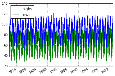
Boo, Pandas and Friends would cry if they saw such a plot.
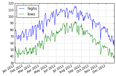
Bringing it Together - Plot
Lets see a smaller slice of time:
phxtemps2['20120101':'20121231'].plot()

<matplotlib.axes._subplots.AxesSubplot at 0x7fca3c66f1d0>
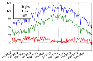
Bringing it Together - Plot
Lets operate on the DataFrame … lets take the differnce between the highs and lows.
phxtemps2['diff'] = phxtemps2.highs - phxtemps2.lows
phxtemps2['20120101':'20121231'].plot()

<matplotlib.axes._subplots.AxesSubplot at 0x7fca3c6ba650>
Pandas Alternatives
- AstroPy seems to have similar data structures.
- I suspect there are others.
References
Thanks! - Pandas and Friends
- Austin Godber
- Mail: godber@uberhip.com
- Twitter: @godber
- Presented at DesertPy, Jan 2015.
- Ipython Notebook